

ETF Liquidation: Sell Before the Cutoff or Wait for Cash?
 zhan chen
A liquidation payment can exceed an ETF’s sale price and still be worth less after a delay. Compare executable sale proceeds with net distributions on one common date, identify the break-even payment, and separate fund expenses from account-specific costs.
A notice that an ETF will liquidate does not establish whether selling now or waiting for the final payment produces the better outcome. The sale route has an executable price and transaction costs. The waiting route has a net entitlement, a payment timetable and uncertainty about both. An old net asset value cannot substitute for any of those inputs.
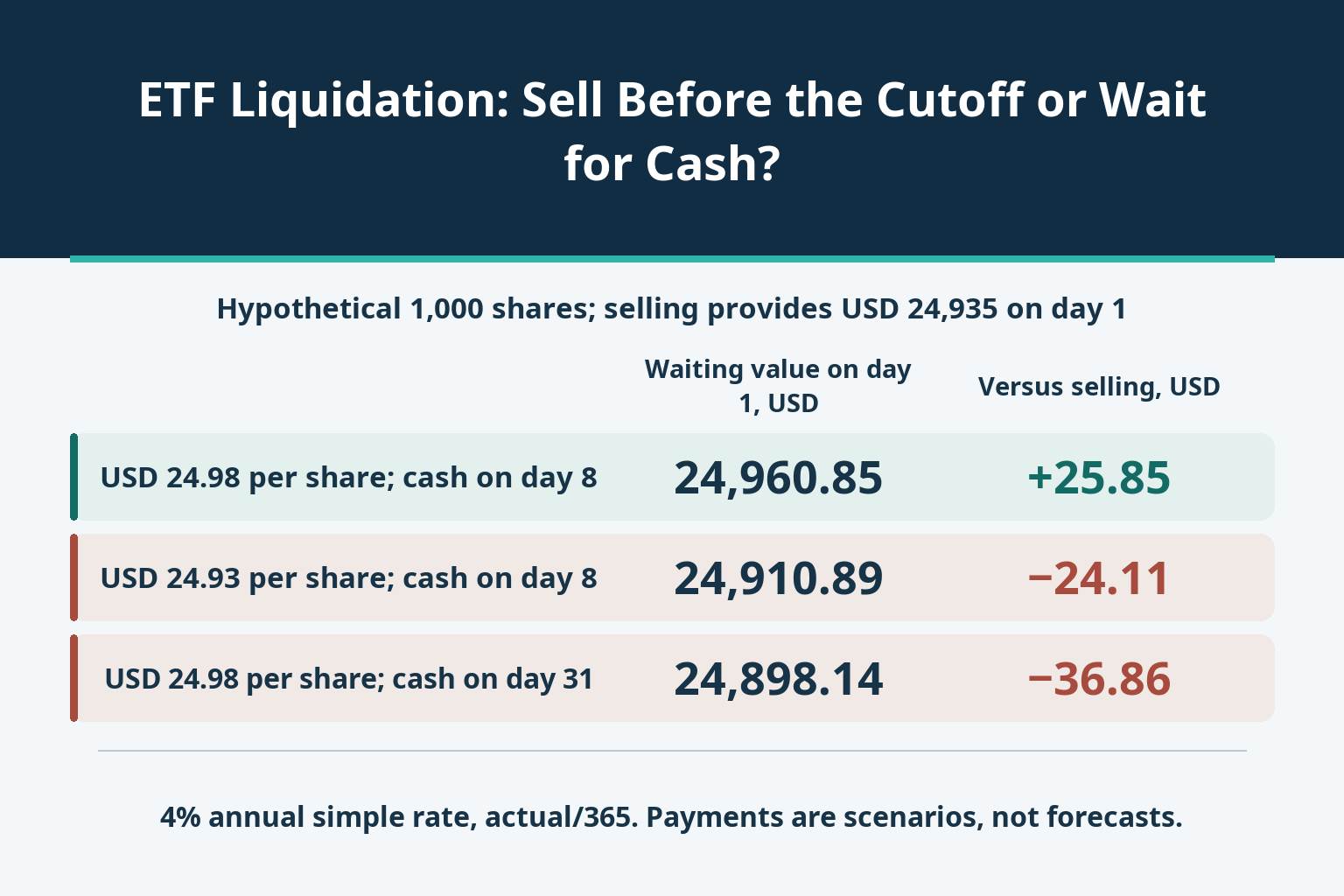
The comparison needs a common cash date. In the hypothetical example below, selling delivers USD 24,935 on day 1. Waiting for USD 24,980 on day 8 is ahead by USD 25.85 when valued on that same day 1 using a specified cash opportunity rate. Delay the identical payment until day 31 and waiting is behind by USD 36.86. Neither result predicts the actual liquidation payment.
Establish what is closing and which deadline matters
A fund liquidation is not simply removal from one exchange, conversion of a share class or merger into another fund. Those events may leave investors with different assets and choices. Start with the issuer’s actual notice, not a screen label saying that an ETF is “closing.” This article uses the mechanics of a hypothetical US-registered ETF distributing cash; another market or legal structure requires its own documents.
Separate the announcement, last trading session, valuation date, issuer payment date and the date cash becomes usable in the investor’s account. They need not coincide. A primary-market creation or redemption deadline is also not necessarily the last opportunity for a retail investor to sell on the exchange.
A real example illustrates the distinction. The June 12, 2026 supplement for the iShares U.S. Select Equity Active ETF, BELT, scheduled exchange trading through the close on or about August 12, a halt before the open on or about August 13, and proceeds to be sent on or about August 17. Its issuer subsequently reported a final trading-day closing price of USD 40.04 and a final distribution rate of USD 39.926954. These are retrospective records, not a price every holder could have executed or an after-tax comparison. Nor does an issuer’s sending date prove when a particular broker made funds available.
Price the sale using a bid that can actually fill
Assume an investor holds 1,000 shares, the fund’s old reference NAV is USD 25.00 and there is sufficient executable bid depth at USD 24.94 for the whole order. The total investor sale fee is USD 5. Net proceeds are therefore 1,000 × 24.94 − 5 = USD 24,935. These are invented teaching inputs, not BELT prices or a broker tariff.
The last trade, midpoint and indicative NAV are not interchangeable with that bid. A smaller displayed size may require several executions at different prices; a limit order may never fill. The distinction between ETF market prices and net asset value matters more than an apparent discount calculated from a stale NAV. Replace the simple sale input with a size-aware execution estimate if the whole holding cannot transact at one price.
The model assumes sale proceeds are usable on day 1. That is an explicit cash assumption, not a universal settlement rule or withdrawal promise. Actual settlement, account restrictions, currency conversion and broker processing can change it. After the relevant trading cutoff, the sale alternative may cease to exist; an earlier displayed quote is not an option that remains available indefinitely.
Define the final payment before subtracting any costs
Let L be the final cash distribution per share after fund-level expenses and liabilities, but before investor-specific taxes or charges. An ETF that is winding down may sell assets and move into cash before its final trading date. Continuing to own its shares therefore need not preserve the original index or strategy exposure throughout the process.
For an independent gross-to-net illustration, assume future asset realisation of USD 25.00 per share and fund costs or provisions of USD 0.02, leaving L = USD 24.98. If future gross realisation is instead USD 24.95 with the same deduction, L is USD 24.93. These are alternative assumed future proceeds, not amounts derived automatically from the old USD 25.00 NAV.
Once L is defined as net, subtracting the USD 0.02 again is an error. Likewise, a reserve is not necessarily a permanent loss: if it is released later, it creates another cash flow. The one-payment example assumes all claims are settled by the final distribution. Actual liquidation notices must establish which expenses are already reflected, whether liabilities remain and whether further distributions are possible.
Put every waiting scenario on the same valuation date
Use day 1, when the sale proceeds become available, for every comparison. The assumed same-currency cash opportunity rate is 4% a year, simple interest, with actual calendar days divided by 365. This is neither an ETF return nor a current deposit offer. It is not a risk-adjusted discount rate that prices uncertainty about the liquidation.
If the payment becomes usable d calendar days after day 1, its common-date value is V = 1,000L ÷ (1 + 0.04d/365). Compare V with USD 24,935. The three rows are independent scenarios, not a sequence of payments. Investor waiting fees, taxes and all other cash flows are excluded at this stage.
| Hypothetical scenario | Net payment per share, USD | Extra calendar days | Nominal payment, USD | Value on day 1, USD | Difference versus sale, USD |
|---|---|---|---|---|---|
| 24.98 per share, available day 8 | 24.98 | 7 | 24,980.00 | 24,960.85 | +25.85 |
| 24.93 per share, available day 8 | 24.93 | 7 | 24,930.00 | 24,910.89 | −24.11 |
| 24.98 per share, available day 31 | 24.98 | 30 | 24,980.00 | 24,898.14 | −36.86 |
In the first row, day 8 means seven additional days. The nominal USD 45 advantage becomes USD 25.85 on day 1; the difference is the specified time value, not a fund charge. The second row holds the date fixed but reduces net asset realisation. The third retains the first row’s USD 24,980 payment but extends the wait to 30 additional days. Its lower common-date value reverses the ranking.
All monetary results are rounded only for display. A positive difference means waiting has the higher value under that row’s inputs; it does not establish that the row is likely. No probability has been assigned, and no compensation for uncertain amounts or dates has been inferred from the 4% rate.
Calculate the payment needed to justify a longer wait
Instead of guessing a final payment, solve for the net amount that ties the two routes: L* = (24,935/1,000) × (1 + rd/365). Here r is the annual simple opportunity rate. Equality means indifference within the model; waiting requires L above the exact threshold to have a strictly higher common-date value.
| Extra calendar days | Annual simple opportunity rate | Break-even net payment per share, USD |
|---|---|---|
| 7 | 0% | 24.93500000 |
| 7 | 4% | 24.95412822 |
| 30 | 4% | 25.01697808 |
With a zero opportunity rate, the threshold is USD 24.935 per share. At 4% and seven additional days it is approximately USD 24.95412822; with 30 additional days it rises to approximately USD 25.01697808. The USD 24.98 scenario clears the first positive-rate threshold but not the second. A final payment above the quoted USD 24.94 bid is therefore not, by itself, enough to make waiting preferable.
The thresholds are not executable quotes and do not reveal the eventual distribution. Use unrounded inputs when testing a close result. A different available cash rate, sale fee, usable-funds date or investor charge changes the boundary; replacing the assumptions is more useful than treating eight displayed decimal places as certainty.
Know when the single-payment comparison stops working
Some liquidations distribute most cash first and retain an illiquid asset or liability reserve. Value each known net payment on the same date using its own timing. Under the same simple cash convention, the waiting total becomes the sum of each payment divided by 1 + r × its extra days/365. Do not collapse all instalments into the first date, and do not silently mark an uncertain residual at zero merely to complete the calculation.
Investor taxes, withholding, acquisition basis and account treatment may differ between a sale and a distribution. Their amounts and payment dates belong in the relevant route’s cash ledger. A US notice’s tax paragraph is not a universal rule for other countries, accounts or fund structures. Investor charges are also distinct from expenses already deducted inside L.
Finally, selling to reinvest in another asset creates different market exposure from waiting in a winding-down fund. A replacement ETF’s unknown return cannot simply be substituted for the 4% cash assumption and called a guaranteed opportunity cost. This controlled example isolates cash amount and timing; market risk, uncertain residuals and personal tax outcomes require additional inputs.
Rebuild the decision from the notice and the account
- Identify the legal event and dates. Confirm that this is a fund liquidation, then record the last trading session, valuation basis, scheduled distributions and any conditions allowing the timetable to change.
- Estimate executable net sale cash. Use the bid and depth for the actual holding, include investor transaction costs, and ask when the resulting funds would be usable rather than relying on a generic settlement label.
- Reconcile the waiting entitlement. Distinguish gross asset proceeds, fund expenses and liabilities, net per-share cash, potential further payments, and account-specific deductions. Avoid charging the same cost twice.
- Choose one date and test separate uncertainties. Compare all cash flows on that date with an explicit annual-rate convention. Vary final net proceeds separately from delays and calculate the break-even payment instead of assigning an unsupported forecast.
- Recheck before the sale window closes. Replace estimates with revised notices, live executable depth and broker information. If the net entitlement or availability date is still unknown, retain that uncertainty rather than reporting a model result as a completed return.
The practical question is not whether liquidation cash looks larger than a screen price. It is whether the possible cash amounts, usable dates and unresolved claims have been defined well enough to compare the available alternatives without confusing NAV, proceeds and time value.


