

Why a 100% Currency Hedge Does Not Guarantee the Local Equity Return
 zhan chen
A hedge can cover all the initial foreign-currency equity value and still leave exchange-rate exposure when share prices move. A fixed-notional EUR/USD model separates forward profit, residual exposure and the effect of resetting the hedge.
“100% currency hedged” needs a denominator and a date. A portfolio can hedge all its initial foreign-currency equity value and still develop a mismatch as the shares rise or fall. If the hedge notional stays fixed, the exchange rate continues to affect the value created or lost during the period.
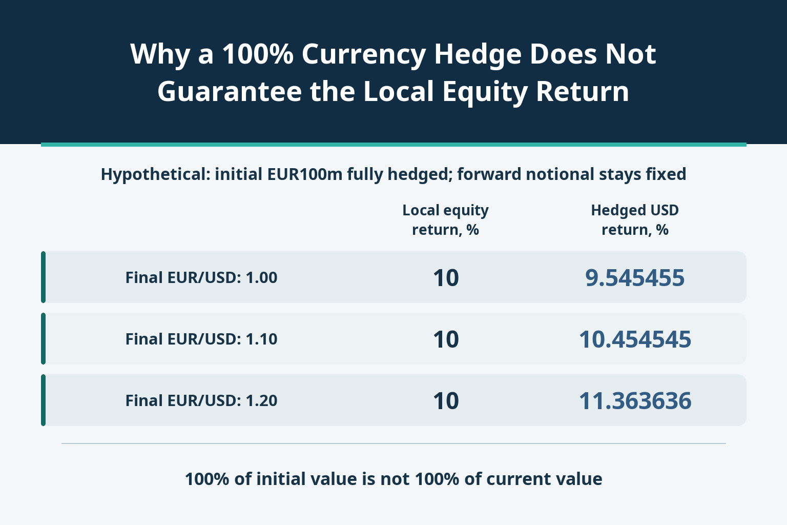
In the hypothetical example below, euro-denominated equities rise 10%. A full initial euro hedge produces a USD return of 9.54545%, 10.45455% or 11.36364%, depending on the final exchange rate. The difference does not, by itself, establish a failed hedge or poor implementation. It follows from exactly what was hedged.
Define what the initial 100% actually covers
Use USD as the reporting currency. The portfolio initially owns equities worth EUR100 million. Spot is 1.10 USD per EUR, making the initial economic value USD110 million. It contracts to sell EUR100 million forward for dollars at 1.105 USD per EUR. The euro notional remains unchanged until maturity.
The stock holdings' trading or valuation currency, the portfolio's reporting currency, a share class's exchange-trading currency and the hedge's target currency are different concepts. A listing in euros does not establish that the product hedges into euros. For an actual product, its own current documents must define the currency basket, reference date and calculation base.
Published index methodologies illustrate both fixed-period and more frequent hedge resets, but an example from one methodology is not a rule for every fund. This is an original one-period model, not a reconstruction of a named index. There are no subscriptions, distributions, taxes, trading costs, cash interest or interim collateral-funding flows.
Keep the equity value and the forward result in separate lines
Let A₀ be the initial EUR100 million equity value and a its local return. Final equity value is A₁ = A₀(1 + a). Let S₁ be the final spot rate in USD per EUR, H the euro forward notional and F the contracted rate of 1.105. All positions reach maturity and perform normally; the final spot is the assumed same-value-date rate used consistently in the model.
The equities are worth A₁S₁ dollars. The forward's signed economic profit or loss at maturity is P = H(F − S₁). Selling euros forward benefits when the contracted dollar rate exceeds the final spot rate, and loses when it is lower. F is a hypothetical contracted rate—not today's quotation, a forecast or a bank fee.
The combined final economic value is V₁ = A₁S₁ + H(F − S₁). Divide by the initial USD110 million to calculate the USD return. The forward term is not the gross dollars received in a physical exchange. Nor does adding it require selling all the equities: if physical delivery is used while shares are retained, obtaining the euros and arranging settlement cash are separate tasks.
The same initial hedge produces five different end states
Keep H at EUR100 million throughout. The table contains five independent hypothetical endings, not five successive trading days. Each row uses the same initial asset value, initial spot and contracted forward rate.
| Local equity return, % | Final spot, USD per EUR | Equities, EUR millions | Equities, USD millions | Forward profit or loss at maturity, USD millions | Combined final value, USD millions | USD return, % |
|---|---|---|---|---|---|---|
| +10 | 1.00 | 110 | 110 | +10.5 | 120.5 | +9.545455 |
| +10 | 1.10 | 110 | 121 | +0.5 | 121.5 | +10.454545 |
| +10 | 1.20 | 110 | 132 | −9.5 | 122.5 | +11.363636 |
| 0 | 1.00 | 100 | 100 | +10.5 | 110.5 | +0.454545 |
| −10 | 1.20 | 90 | 108 | −9.5 | 98.5 | −10.454545 |
In the first row, the equities rise to EUR110 million but the euro falls to USD1.00. The equities alone are worth USD110 million, exactly the initial dollar value: the unhedged USD return would be zero. The forward earns USD10.5 million, bringing combined value to USD120.5 million and the hedged return to 9.54545%.
If the same EUR110 million of shares is instead worth USD1.20 per euro, the equities translate to USD132 million. The forward loses USD9.5 million, leaving USD122.5 million overall. Examining only that derivative loss would miss the currency gain on the equities; examining only the equities would omit the hedge.
The last row makes the opposite point. With local equities down 10% and final spot at 1.20, the combined value is USD98.5 million, a USD return of −10.45455%. Currency hedging has not insured the equity portfolio against falling share prices.
The missing term is the return on the newly created exposure
For a full initial hedge, H = A₀. Define the spot return x = S₁/S₀ − 1 and the forward-rate component f = F/S₀ − 1. The return identity becomes R = a + f + a×x. It is not generally just the local equity return plus the forward-rate component.
Equivalently, R = a(S₁/S₀) + f. The unhedged USD return is (1 + a)(1 + x) − 1. These expressions use the same initial dollar denominator: the hedge removes the currency effect on the initial euro amount, not on every change in that amount during the period.
Here f is 0.454545% for the modelled period. In the first row, a is 10% and x is −9.090909%. Their product subtracts 0.909091 percentage points from 10% + 0.454545%, producing 9.545455%. That subtraction is an interaction between the asset return and the exchange-rate move, not an extra fee.
The same mechanism appears in euro amounts. Residual notional is A₁ − H = A₀a. After a 10% equity gain, EUR10 million is outside the fixed hedge, and H/A₁ is only 90.90909%. After a 10% decline, the hedge exceeds the equity value by EUR10 million and the ratio is 111.11111%. These ratios refer only to the equities' euro market value, not total fund assets or a regulatory net-exposure measure.
A useful control is a = 0. With equity value unchanged at EUR100 million, the mismatch disappears and R = f regardless of S₁ under these assumptions. This identity validates the model; it is not a promise about a real fund with cash flows, costs or a different hedge schedule.
A 50% initial hedge may not remain a 50% current hedge
Now keep the first ending—local equities up 10% and final spot at 1.00—but vary the initial fraction h. Set H = hA₀. The general return is R(h) = (1 + a)S₁/S₀ + h(F − S₁)/S₀ − 1.
| Initial hedge ratio, % | Forward notional, EUR millions | Forward profit or loss at maturity, USD millions | Combined final value, USD millions | USD return, % | Final notional / equity value, % |
|---|---|---|---|---|---|
| 0 | 0 | 0 | 110 | 0.000000 | 0.000000 |
| 50 | 50 | +5.25 | 115.25 | +4.772727 | 45.454545 |
| 100 | 100 | +10.5 | 120.5 | +9.545455 | 90.909091 |
Hedging EUR50 million earns USD5.25 million on the forward and gives a combined value of USD115.25 million, a 4.772727% USD return. Yet the final hedge covers 50/110, or 45.454545%, of the equity value. For the initial full hedge, the corresponding final ratio is 100/110, or 90.909091%.
Higher initial coverage improves the result in this particular weakening-euro ending. It is not a universal ranking of strategies. The other ending with a strengthening euro shows why retaining more exchange-rate exposure can instead help the translated equity value. Choose the intended exposure before observing the outcome, rather than declaring whichever hedge won the scenario optimal.
Resetting the hedge changes the strategy, not just the spreadsheet
It is tempting to insert the known final EUR110 million into the initial hedge and call that perfect protection. That uses future information. A real adjustment can only use holdings and prices available at the adjustment date, and it requires another trade with its own forward rate, maturity and costs.
More frequent resets can reduce newly developed notional mismatches, but this one-period table does not prove continuous elimination of currency exposure or the lowest implementation cost. Subscriptions, redemptions, dividends, portfolio trades and tolerance bands also alter the base. An announced target and an observed current ratio can differ without a mandate breach; the current methodology determines what was required.
Timing matters for valuation too. The expression H(F − S₁) is a maturity result. For a forward's value before maturity, the remaining-term quotation and discounting must be considered. Attributing every tracking difference to forward points overlooks these valuation, implementation and cash-flow distinctions. Hedging the chosen currency value also leaves companies' own international revenue and cost sensitivities inside their share prices.
Five checks for interpreting a hedged return
- Identify trading, reporting, asset and hedge-target currencies separately. Read the product's actual currency allocation rules rather than infer them from its listing.
- Find the date and base behind the target percentage, the permitted range and the reset schedule. Compare like denominators.
- Reconstruct the actual notional, contracted forward rate and same-value-date final conversion rate. Distinguish maturity economics from pre-maturity valuation and gross delivery cash.
- Reconcile equity returns, hedge profit or loss and changes in holdings or cash. Add costs, taxes, collateral funding and distributions where applicable.
- Test both rising and falling equity values and both exchange-rate directions. Evaluate the intended residual exposure, not just whether one realized period beat the unhedged alternative.
The central question is not whether a label says 100%. It is whether the notional, observation date and reset rule match the exposure the investor expects to remove. Once those are explicit, a return different from the local equity return becomes something that can be reconciled, rather than automatically blamed on a defective hedge.


